Watching a language model denoise instead of type
Written with Claude. I wrote the ideas and structure; Claude helped refine the prose.
Every autoregressive LLM you’ve used writes the same way: one token at a time, strictly left to right, each token conditioned on the ones before it. Diffusion language models don’t work like that. They start a whole block of text as pure noise and denoise it, revealing tokens in parallel over a handful of steps, roughly in order of confidence rather than reading order. DiffusionGemma does exactly this, and I built a small visualizer so you can watch it happen. It’s worth seeing.
That’s the model answering “Write a six-line poem about the ocean where the lines start with the letters O, C, E, A, N, S in that order.” Notice what it does first. It doesn’t write line one and move on. It scatters the line-start letters across the block before most of the lines even exist, then fills in the middles. That ordering is the whole story.
What the visualizer shows
The visualizer wraps the model in a Gradio app and renders every denoising step as a frame. It hands back the intermediate canvas at each step, so what you’re seeing is the model’s actual state mid-denoise, not a replay. The color coding is the key to reading it:
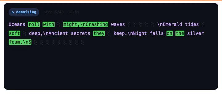
- Gray
░: still noise, a masked position the model hasn’t revealed yet. - Green: revealed this step. These are the tokens the model just became confident about.
- Purple: draft tokens from earlier steps, sitting on the canvas but not committed yet.
- White: committed output. Locked in.
Watch the green flicker around the canvas and you’re watching the model’s confidence order directly. It doesn’t sweep left to right like a cursor. It lands wherever the model is most sure, the purple drafts settle, and then a block commits to white.
The interesting part: scaffolding before content
Here’s the thing that changed how I think about it. Run a structured prompt, one with constraints on form and not just content, and you can watch the model put down the scaffolding before it fills in the substance. The constraint markers show up early, as anchors, and the free text denoises around them.

The acrostic above is the cleanest example: the O/C/E/A/N/S line-starts show up before the lines they head. The model is basically committing to the skeleton of the answer first, then solving the much easier sub-problem of “write a plausible ocean line that starts with C” against anchors that are already fixed. An autoregressive model has no equivalent move. It would have to plan the acrostic implicitly and hope each line’s first token landed right as it streamed past.
The code prompt makes the same point in a different register:
Asked for “a Python function is_palindrome(s) with a docstring and three doctest examples,” the model denoises a skeleton first, the def line, the docstring quotes, the >>> doctest prompts, and only then fills in the bodies. The structure of a correct answer shows up before its details, which is a lot closer to how a person writes code than to how an autoregressive model emits it.
The other demo prompts are picked for the same reason. Each one has structure that becomes visible as scaffolding:
| Prompt | Scaffolding that appears early |
|---|---|
| Acrostic ocean poem (O, C, E, A, N, S) | The six line-start letters, before the lines |
| “Why is the sky blue? In exactly three sentences.” | Sentence boundaries / the three-sentence shape |
is_palindrome(s) with docstring + doctests |
def / docstring / >>> skeleton before bodies |
| Eight planets, one per line, each a fun fact | List markers across the whole block at once |
| 100-word story that begins and ends with the same sentence | Both fixed endpoints, before the middle exists |
| Haiku about ML + explanation of its 5-7-5 structure | The three-line haiku shape |
The story prompt is the one I find most striking: when the task needs the first and last sentence to match, the model can pin both ends of the canvas before the middle has been written at all. That’s a generation order an autoregressive model simply can’t produce.
One caveat. I’m describing what the canvas shows, the order in which positions get revealed on these prompts. I’m not making any claim about the model’s quality, its accuracy next to other models, or its speed.
What a diffusion language model is
So how does it pull that off? It comes down to how the text is factorized. An autoregressive model factorizes it as a product of conditionals: P(token | everything to the left). It samples position 1, appends it, samples position 2, and so on. The output grows one token at a time, and once a token is out you can’t revise it.
A diffusion language model factorizes differently. It works over a fixed-length block, a “canvas” of positions that starts out entirely masked: every slot is noise, drawn here as ░░░░. Then it runs a small number of denoising steps. At each step the model looks at the whole partly-revealed canvas and decides which masked positions it’s confident enough to fill, committing several at once. The ones it’s sure about get revealed early. The ambiguous ones wait for more context to settle around them. After enough steps the canvas is fully denoised and becomes the committed output. Longer outputs just run as several blocks in sequence.
The upshot is that generation is parallel within a block and not left to right. The model can drop a token near the end of the canvas before it has filled the middle, because its confidence about that token doesn’t depend on reading order.

DiffusionGemma is a 26B-parameter mixture-of-experts model with roughly 4B parameters active per token, which is the “26B-A4B” in its name. MoE means most of those 26B weights sit idle for any given token: a router picks a small subset of experts to actually run, so you pay download and memory for 26B but compute closer to 4B.
The motivation: speed, and therefore cost
The reveal order is what makes the visualizer fun to watch, but it isn’t why Google is pouring effort into this architecture. The reason is throughput. Because a diffusion model commits several positions per denoising step instead of one token per forward pass, it can emit a lot of text per unit of compute. DeepMind’s own framing is blunt about it: DiffusionGemma “generates up to 4x-5x faster token output on NVIDIA GPUs (achieving over 1,000 tokens per second on a single H100),” and it gets there by “generating 256 tokens in parallel with each forward pass.” So the “4x” number I’d half-remembered is real, and if anything conservative: Google states 4x to 5x. The model card puts the mechanism in concrete terms, “generating 15-20 tokens per forward pass, unlocking per user generation speeds exceeding 1100 tokens per second” at low batch size on an H100 (Google AI model card). This lineage goes back to Gemini Diffusion, the experimental DeepMind model shown earlier, which clocked 1,479 tokens per second and was pitched as “significantly faster than even our fastest model so far.”
The mechanism is exactly the parallel decoding the visualizer makes visible. An autoregressive model is bottlenecked on memory bandwidth: every token requires its own forward pass, streaming the weights through the accelerator one step at a time, and you can’t start token n+1 until token n exists. A diffusion model fills many positions in a single pass over the whole canvas, so DeepMind describes it as “shifting the decode bottleneck from memory-bandwidth to raw compute”. That’s the same scaffolding-then-content behavior from earlier, seen from the hardware’s side: the parallelism that lets the model pin both ends of a story before the middle is also what lets it produce more tokens per pass.
Here’s where I’ll mark the line between what Google says and what I’m inferring. Google states the speed; it does not, in the material I found, put a price on it. But the cost consequence seems hard to avoid. If you can serve four to five times as many tokens from the same GPU in the same wall-clock time, your cost per token falls by roughly that factor, and the model card is explicit that this design is “optimized for small batch size inference”, the low-latency, single-accelerator regime rather than huge batched fleets. So my read, and I’d flag it as interpretation rather than a cited claim, is that the payoff lands hardest on small, cheap, high-volume models. For a frontier model the quality gap still dominates the decision. For a small workhorse model doing structured, repetitive jobs at scale, where the output is short and the structure is regular, the same per-token speedup turns directly into a serving-cost advantage. A faster small model is a cheaper small model, and cheap-at-volume is exactly the niche a 4B-active MoE like this one is built to fill.
Running it yourself
The model is google/diffusiongemma-26B-A4B-it (Apache-2.0, ungated), and the visualizer is on GitHub at alainbrown/diffusion-visualizer. It runs on Apple silicon.
On an Apple-silicon Mac you can run the real model natively with the pre-quantized 4-bit checkpoint mlx-community/diffusiongemma-26B-A4B-it-4bit (~16.6 GB to download, and it fits a 24 GB Mac). It uses mlx-vlm’s stream_generate with diffusion_show_unmasking=True, which surfaces the per-step canvas. This is what I recorded the videos on, locally on a Mac. MLX uses Metal, so it runs natively on the host rather than in a container.
It’s in the repo. Clone it, run it on an Apple-silicon Mac, and the demo prompts above are one click away.
Why watching it matters
You can read the sentence “diffusion language models generate in parallel, not left to right,” nod, and still walk around with an autoregressive mental model where text comes out like a typewriter. Watching the acrostic letters appear before their lines, or both ends of a story pin themselves before the middle exists, breaks that picture in a way the sentence never did. The model isn’t typing faster. It’s solving the problem in a different order, committing to the shape of an answer and then working out the details against it.
That’s the part worth seeing for yourself. Pick a prompt with some structure, hit denoise, and watch where the green lands.